
learning notes about automl
Introduction
machine learning
- the learning algorithm outputs a model whereas the model outputs predictions
- the learning algorithm take in pre-processed data and output a model
- then the model is different in the sense that it takes in new inputs or just inputs and its outputs are predictions for those inputs
- difference between parameter and hyperparameter
- the model is often associated with parameters denoted by the symbol and parameters control the behavior of the model which is determined by the learning algorithm, so the learning algorithm often outputs these parameters and we do not have to think about them ourselves as human experts
- the learning algorithm also has parameters but to distinguish these from the model parameters we call them hyperparameters. It control the learning outward and these are often determined by the humans.
- example:
- parameters: the thresholds in every node and maybe the rows that we use to go either left or right (for a neural network and in a decision tree)
- hyperparameter: something like the learning rate, the momentum value and so on (when trained with gradient descent)
role of the human experts
- what data processing steps: cleaning, feature engineering like what feature extraction and deed into the learning algorithm etc
- what learning algorithm do we use, svm, logistic regression, neural network
- what hyperparameters do we use for the given learning algorithm (hyperparameters selection)
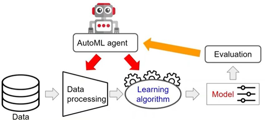
automated machine learning = automating one or more of these things
ml => automl
when determine data processing, learning algorithm and hyperparameters:
we introduce an automl agent which is either responsible for part of the choices that have to be made or it can fully replace the human and be responsible for making all of these choices.
why automate ml
choice of preprocessing, learning algorithm and hyperparameters is crucial for achieving good performance
- finding good setting for these components requires expert domain knowledge so this is something often done by data scientists who understand the machine learning algorithm and understand the influence of the different choices on the performance
- takes a lot of tedious effort and is expensive to actually find correct settings for all of these components in order to be satisfied with the performance
- having a human finding good settings for these components maybe suboptimal
use automl we can
no longer need expert domain knowledge
increase the wide applicability and lower the threshold for actually using these techniques
better performance
auto ml
consists of 3 parts:
- search space: all of the different hyperparameters values maybe pre-processing steps etc over which the agent can search
- search algorithm: determines how it is going to search through this search spase
- evaluation mechanism: what we do in search i s we want to try to maximize the performance, so we need to have some kinds of evaluation mechanism
- that allows us to distinguish candidate solutions in the search space from each other
- and which allows us to guide the search towards more and more promising or well-performing methods
overview
overview$^{[1]}$, we only care about the part of neural architecture search (NAS)
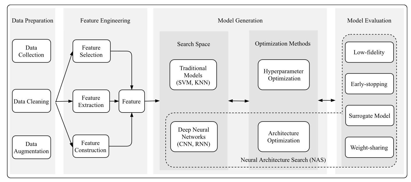
- search space
- architecture optimization
- evolutionary algorithm
- reinforcement learning
- gradient descent
- bandit-based
- successive halving
- hyperba
- surrogate model-based optimization
- EGO/TB-SPO
- bayesian optimization (BO)
- Gaussian process (GP)
- random forest (RF)
- tree-structured parzen estimator (TPE)
- bo-based hyperband (BOHB), combines the strengths of TPE-based BO and hyperband
- neural networks
CASH vs HPO
definition of CASH
CASH = combined algorithm selection and hyperparameter optimization
given:
- $\mathcal{T}$: task we want to solve
- $\mathcal{D}_{train}$: the training data
- $\mathcal{L_T}$: the loss function => performance metric which measures how poorly our solutions are performing
- (we want to find the best algorithm and the best hyperparameters)
- $\mathcal{A}$: the space of all algorithms over which we search
- $\Theta$: the space of hyperparameters over which we search
we want to find:
$$
A^*, \theta^* = \arg\min\limits_{A \in \mathcal{A}, \theta \in \Theta} \space \mathbb{E}\mathcal{pT} [\mathcal{L_T}(A_\theta(D{train}))]
$$
where
hyperparameter vector $\theta = [\theta_1 \theta_2 \dots \theta_n]$
- e.g. , [learning rate, momentum, use_batch_norm]
$A_\theta(D_{train})$ means the output of learning algorithm, namely the model (the algorithm takes in the data and outputs a model)
$\mathcal{L_T}(A_\theta(D_{train}))$ means the loss of the model on a given data point
$\mathbb{E}_\mathcal{pT}$ means the expected or mean loss of the model
in short, we want to find the best of algorithm and hyperparameter such that we minimize…
definition of HPO
based on definition of CASH, assume that the algorithm is given so we no longer want to find a best algorithm
given a certain learning algorithm, we only want to find the best hyperparameters:
$$
\theta^* = \arg\min\limits_{\theta \in \Theta} \space \mathbb{E}\mathcal{pT} [\mathcal{L_T}(A_\theta(D{train}))]
$$
relationship
HPO = CASH when including the algorithm as “hyperparameters”
=> 将【算法】作为超参数包含在我们的结果$\theta$中
GS vs RS
grid search
definition
- define sets of values you want to try for some (or all) hyperparameters, evaluate all possible combinations => traversal
value sets:
$$
v(\theta_1) = { 0.1, 0.01, 0.001 }\
v(\theta_2) = { 0.99, 9.9, 0.8 }\
\dots\
v(\theta_n) = { True, False }
$$
evaluate:
$$
v(\theta_1) \times v(\theta_2) \times \dots \times v(\theta_n)
$$
this evaluation procedure is often done on a validation set, not training set because that will give us a biased view and may lead to over-fitting
pros and cons
- pro
- simple
- easy to parallelize
- cons
- waste of compute when one or more hpms are not important
- scalability (exponential growth number of combinations)
- how to define the grid: how do we know that the values that we put in the value sets are actually good values to try out
- this is what random search actually kind of solves
random search
definition
define probability distributions on ranges of values for every hyperparameters, draw hyperparameters configurations and evaluate
sample from the range and sample according to some kind of probability distribution that we have defined over this range
distributions:
$$
p(\theta_1) = LogUniform(0.001, 0.1)\
p(\theta_2) = Uniform(0.8, 0.99)\
\dots\
p(\theta_n) = Categorical({ True, False })
$$
we transform both of these two values (minimum and maximum) into log space, we sample in the log space and then we transform the sampled values back to the original space
evaluate M configurations:
$$
\theta \sim p(\theta_1, \theta_2, \dots, \theta_n)
$$
we evaluate samples from the joint distribution
in order to sample one configuration, we have to sample the first value from the first distribution, the second value from the second distribution etc
so we need to sample in total from M times in n distributions
pros and cons
- pros
- simple
- easy to parallelize
- can set a budget of function evaluations (evaluate M hyperparameter configurations)
- theoretical guarantees of convergence with proper ranges
- not really has any meaning in practical scenarios
- cons
- not data efficient
- still expensive
relationship
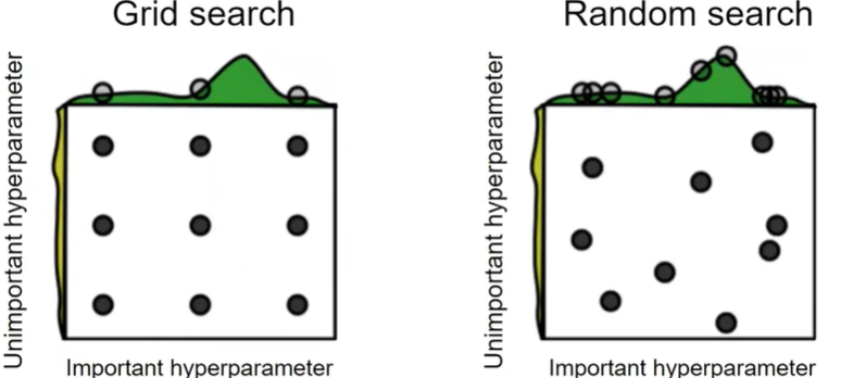
random search is more efficient when there are unimportant hyperparameters (better coverage)
Successive Halving vs Hyperband
downside of gs and rs: every hyperparameters configuration is fully trained => expensive
we can detect early on that a configuration will be bad and discard it, so techniques to do this:
- successive halving
- hyperband => the extension of successive halving
successive halving
idea
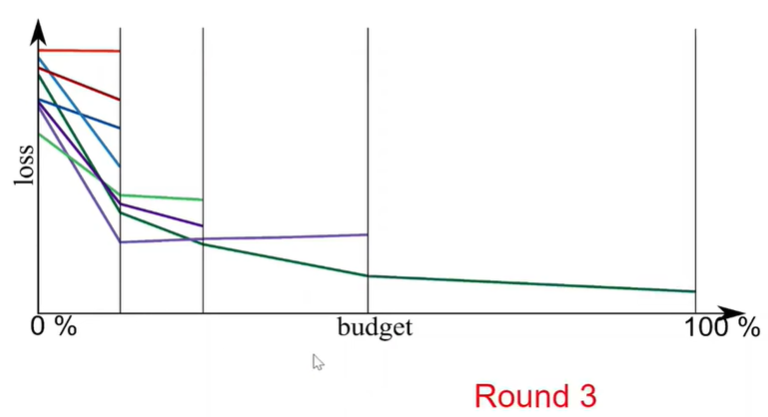
on the x-axis we have compute budget which can think of as the total number of epochs
on the y-axis we have the performance metric, here is loss
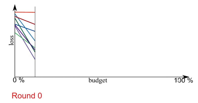
in round 0 we start a randomly sampled configuration.
(after making a number of training steps we evaluate all configurations in this round) => throw the worst half off and continue training the best half
- we simply throw away the worst half of these configurations
- we stop training them and we continue training the best half
definition
start a set of $n$ random initial configurations ${ A_\theta^{(i)} }^n_{i=1}$ and a budget $B$
every round the candidate pool size is divided by $\gamma$ which means halving rate
we only perform $log_\gamma(n)$ rounds
budget is divided uniformly rounds
- but because we throw away configurations in every round what this basically means is that every configuration is assigned more budget per round
- consequently we assign exponentially more budget to good configurations
example
- number of initial configurations n = 64. total budget B = 384, halving rate $\gamma$ = 2
- computation metric
- round => k
- number of candidate pool in this round => $S_k$
- budget in this round per configuration => $r_k$
- procedure
- $log_2(64) = 6$, so we only need to perform 6 rounds, namely k = { 0, 1, 2, 3, 4, 5 }
- $\gamma = 2$, so $S_k$ = { 64, 32, 16, 8, 4, 2 }
- since budget is divided uniformly rounds, we have 6 rounds here, the budget of each round is 384/6 = 64. then we divide the total budget per round by $S_k$, namely 64/$S_k$, so $r_k$ = {1, 2, 4, 8, 16, 32 }
hyperparameters
higher budget => higher budget per configuration (more informed decisions and more compute times)
higher halving rate => more aggressive pruning (could be too aggressive and disregard the best candidate early on, imagine a configuration which starts learning quite slow and only after a certain number of epochs starts to really maximize the performance)
pros and cons
pros
- allow us to work with fixed budget
- good experical results
- strong theoretical foundations
- parallelizable
cons
learning curves can cross (good candidates to be discarded early)
n / B trade-off, given a fixed budget B
- larger n => smaller amount of time per config
- smaller n => larger amount of time per config
- we do not know which works best => this is what hyperband actually solves
hyperband
idea
running successive halving different times with different values of n
- firstly, it does a bracket of successive halving using a large number of initial configurations
- then it simply randomly sample another set of initial configurations and this time lower the amount than in our previous round
- we again decrease the candidate pool size until we are in our final bracket which is equivalent to a random search
definition
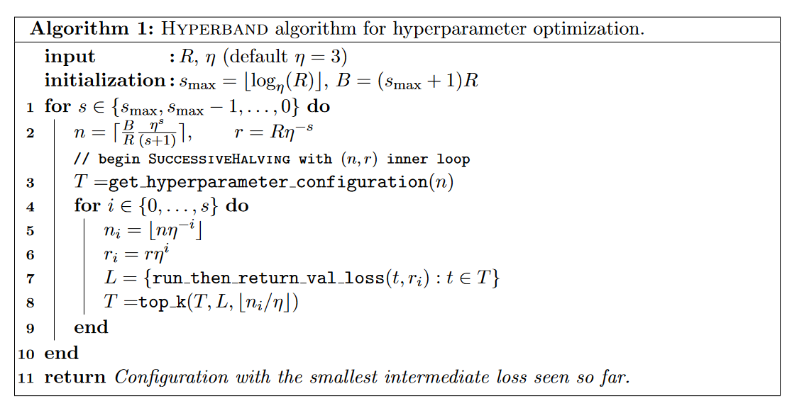
perform different successive halving with hyperband (here we call bracket) $s_{max} + 1$ times with various initial candidate pool size $n$ (in essence performing a grid search over feasible value of $n$) for a fixed budget $B$
- start with large $n$ (we do quite some exploration, but less time per configuration), subject to the constraint that at least one configuration is allocated R resources.
- every consecutive bracket, reduce n (we decrease the n which means that we will get more time per configuration but a smaller number of configurations and this also leads to less exploration) until the final bracket, s = 0, in which every configuration is allocated R resources (this bracket simply performs classical random search)
conclusion => there are two components to hyperband
- the inner loop invokes successive halving for fixed values of n and r
- the outer loop iterates over different values of n and r
hyperparameters
R: maximum resource that can be allocated to a single configuration within a round of successive halving
$\gamma$: control proportion or discarded configurations every round
example
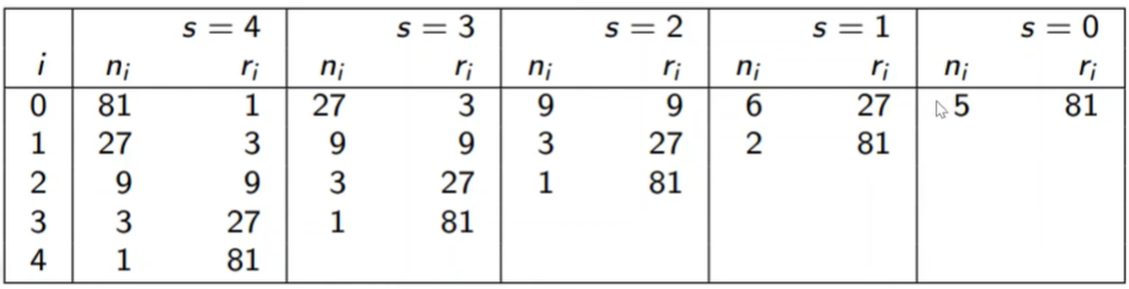
- various brackets, with R = 81 and $\gamma = 3$
- firstly, we consider the number of different brackets we need to perform, it’s $s_{max} + 1 = log_{\gamma}(R) + 1 = log_3(81) + 1 = 4 + 1 = 5$. and $B = (s_{max} + 1) R = 5R$
- In the $s_{max}$ bracket: since we have a fixed budget R = 81, according to the algorithm, we start with a large number of configurations n, so here n is equivalent to R, namely 81 (or we can compute according to the equation $n = \gamma^{s_{max}} = 3^4 = 81$). so in the round zero, budget for each configuration $r_i$ is R/n = 81/81 = 1. then in the next round of this bracket we perform the algorithm as successive halving until the budget for each configuration in the round is equal to R
- then in the third bracket, we decrease the initial number of configurations using given halving rate $\gamma = 3$, so n of round zero of second bracket should be $81 / 3 = 27$ (we can compute according to the equation $n = \lceil \frac{5R}{R} \frac{\gamma^s}{s+1} \rceil = \lceil 5 \frac{3^3}{3+1} \rceil = 34$, so we chose 27 because 27 < 34 and the output of $log_3(27)$ is an integer). note that we have fixed maximum budget for all configurations in each round, still be R = 81, so this time the budget for each configuration $r_0 = R/n_0 = 81/27 = 3$
- in the second bracket, we perform as before. the initial value of $n_i$ and $r_i$ should be 27/3=9 and 81/9=9 ($n = \lceil \frac{5R}{R} \frac{\gamma^s}{s+1} \rceil = \lceil 5 \frac{3^2}{2+1} \rceil = 15$, so we chose 9)
SMBO
surrogate model-based optimization
limitation of techinique so far
- they randomly select initial candidates to evaluate
- but if we have already evaluated a set of candidates, we can do better than random selection
- predict promising regions based on history of observations
- we could fit a model to our previous observations and then use this model to predict the most promising regions or the most promising hyperparameter configurations
idea
learn a surrogate model that for every configuration $\theta \in \Theta$:
predicts the loss or performance
provides a measure of uncertainty about the prediction
loosely speaking, the surrogate models $P(y \vert \theta)$, where y denotes the performance and $\theta$ denotes a given hyperparameter
so we need to update the surrogate model sequentially as new observations (tried configuration, performance) arrive
and we use the surrogate model to select new promising configurations to evaluate
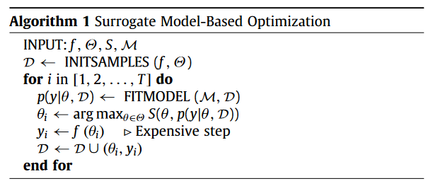
- symbol explanations
- evaluation function => $f$
- search space => $\Theta$
- acquisition function => $S$
- probability model => $M$
- dataset $D$, it includes many sets of samples $(θ_i, y_i)$ where $\theta_i \in \Theta$ and $y_i$ denotes the performance of $\theta_i$
instantiation
- bayesian optimization
- start with a prior distribution, namely start with initial surrogate model and as data points come in and as we try out more configuration and observe their performances
- we repeat: update our beliefs about the loss surface so that we update our surrogate model
surrogate model
Gaussian process (good confidence bounds, however only numerical hyperparameters)
- face some challenge when having categorical hyperparameter, it’s not easy to incorporate it
random forest (categorical and conditional hyperparameters)
- categorical => a boolean flag where we want to use batch normalization in a neural network
- conditional => hyperparameters that are only defined if some other hyperparameter is satisfied with some constraints. suppose we have a neural network and we have one hyperparameter that is the number of nodes in layer number 3, now for this hyperparameter to actually carry any meaning we need to have the other hyperparameter value which is the number of layers to be larger or equal than 3 because otherwise this one hyperparameter does not make any sense.
BO
referencing the blog post$^{[2]}$, this part add some understanding and other supplementary content related to mathematics
似然估计与其函数
回顾总结一下遗忘的知识:
- 先验概率:在结果发生前就获得的、根据历史规律确定原因的概率,即 $p(因) = p(x)$;
- 后验概率:已知结果,猜测原因,即 $p(因 \vert 果) = p(x \vert y)$
- 似然估计:已知原因,猜测原因对应的结果的概率,即 $p(果\vert 因) = p(y \vert x)$
联合概率密度函数:$p(x, y) = p(x \vert y)p(y) = p(y \vert x)p(x)$
贝叶斯公式:$p(x \vert y) = \frac{p(y \vert x)p(x)}{p(y)} = \frac{p(y \vert x)p(x)}{\int p(y \vert x)p(x) dx}$,根据似然概率和先验概率求后验概率。
而似然函数是用于描述观测数据与某个概率模型之间的关系的函数。假设有个概率模型,由一组未知参数 $\theta$ 描述,有一组观测数据 $D_0$,那么似然函数 $L(\theta | D_0)$ 就表示在给定数据 $D_0$ (因)下,参数 $\theta$ (果)取某个值的概率。
$$L(\theta|D_0) = P(D = D_0|\theta)$$
$P(D=D_0|θ)$ 表示在参数 $θ$ (果)的条件下,数据 $D_0$ (因)出现的概率,后验概率。
通过最大化似然函数,我们可以找到参数 $θ$ 的最优估计值,也即使观测数据出现概率最大的参数值。
problem description
$$
x^{*} = arg\space \max\limits _{x \in \mathcal{X}} f(x)
$$
- 这里 $\mathcal{X}$ 是超参数空间,比如对于一个随机森林模型,这里 $\mathcal{X}$ 就是模型和模型对应的参数,即 { random_forest, n_ estimators, max_depth }。
- $f(x)$ 是参数空间到我们感兴趣的一个指标的映射函数,如回归问题中的MSE或者分类问题中的accuracy和AUC指标。注意不是数据集到预测结果的映射,而是**在某个数据集下,某个模型及其相关的参数$\mathcal{X}$到我们关心的指标的映射 **,如 $f(x): \mathcal{X} \rightarrow acc$。
- 可以认为$f(x)$是一个黑盒函数,其计算代价很高,解决该优化问题被称为黑箱优化。
- 注意$f(x)$的凹凸性质,没有一阶或高阶导数,不能通过梯度下降或者牛顿相关算法进行求解,但我们知道$f(x)$是连续函数,因此可以使用高斯回归过程对$f(x)$进行建模。
iterating method
对于 $y=f(x)$,假设有个先验概率,每次有新的数据 ${ x_{data}, f(x_{data}) }$,求出y的后验概率 $p(y | (x_{data}, f(x_{data})))$,并把这个后验概率作为下一条数据的先验概率,如此迭代更新。
重点是我们需要一个规则来找到基于当前情况的下一个迭代数据 $x_{next}$。所以我们需要基于当前 $y$ 的后验概率,定义一个acquisition function: $a_n(x | data)$,$x \rightarrow R$,这个函数用于计算在当前情况下不同的数据 $x$ 对 $y$ 的作用,从而去选择新的下一条数据 $x_{next}$ 以最大化 $a_n$。
algorithm procedure
给定一个 $y=f(x)$ 的先验概率 $p_0$,最大迭代次数 $N$
随机初始化 $n_0$ 个点,并得到 $n_0$ 个点结果,即
$$
{ (x_1, f(x_1)), (x_2, f(x_2), …, (x_{n_0}, f(x_{n_0}))) }
$$利用初始化的$n_0$个点,更新先验概率,并更新 $n \leftarrow n_0$
当 $n \leq N$ 时:
- 根据当前的后验概率 $p(y | { (x_1, f(x_1)), (x_2, f(x_2), …, (x_{n_0}, f(x_{n_0}))) })$ 来计算 $a_n (x)$
- 选择能够最大化 $a_n(x)$ 的点作为 $x_{n+1}$。注:这一步是重点,该如何找到下一个迭代点 $x_{next}$ 以及过程中如何对 $p(y \vert x)$ 和 $p(y|x_{next})$ 进行建模
- 将新的点 $x_{n+1}$ 带入得到 $f(x_{n+1})$ ,会非常耗时
- $x \leftarrow n + 1$
返回评估过的数据中使得 $f(x)$ 最大的点 $x^{*}$
GP
Gaussian Process Regression
主要解决前面提到的贝叶斯推断中的两个重点问题:1)概率建模;2)下一个迭代数据点的确认。
probability modeling
多维正态分布的似然函数
对于贝叶斯优化的初始化数据 ${ (x_1, f(x_1)), (x_2, f(x_2), …, (x_{n_0}, f(x_{n_0}))) }$,假设多维似然函数 $L$ 服从多维正态分布,后验概率密度为:
$$
p(y) = \left( \begin{matrix} y_1 \ y_2 \ … \ y_{n_0} \end{matrix} \right) \sim N\left( \left(\begin{matrix} u_0(x_1) \ u_0(x_2) \ … \ u_0(x_{n_0}) \end{matrix}\right), \Sigma_{n_0 * n_0}\right)
$$
$$
\Sigma_{n_0 * n_0} = \left [ \begin{matrix} k_{11}&\dots&k_{1 n_0} \ \vdots & \ddots & \vdots \ k_{n_01} & \dots & k_{n_0n_0} \end{matrix} \right]
$$
注意这里 $\Sigma$ 是大写的 $\sigma$,一般来说 $\Sigma$ 是一个 $n_0 \times n_0$ 的协方差矩阵,这个矩阵描述了 $n_0$ 个数据两两之间的相关性。其计算方法:
- 对角线元素 $\Sigma_{ii} = Cov(x_i, x_i) = K(x_i, x_i)$;
- 非对角线元素 $\Sigma_{ij} = Cov(x_i, x_j) = K(x_i, x_j)$
这里对协方差矩阵的建模采用了核函数 $K(·,·)$,不同的核函数又会有不同的计算公式,如:
- 线性核函数:$K(x_i, x_j) = x_i^T x_j$,对两个向量做内积
- 高斯核函数:$K(x_i, x_j) = e^{-\frac{||xi - xj||^2}{2σ^2}}$。
- $\sigma$ 是核函数的带宽参数,控制着核函数的平滑程度,$\sigma$ 越小,相关性变化越剧烈。
- 公式反映了不同变量 $x_i$ 和 $x_j$ 之间的相关性,距离才用了 $L2$ 距离,距离越近($||x_i - x_j||^2$ 越小),相关性越强($\Sigma_{ij}$ 越大),由公式得对角线元素为1。
- 该核函数满足了对称性且保证了协方差矩阵为非负正定矩阵(是一个对称矩阵,并且对于其中任意非零向量 $x$,$x$ 与该矩阵的乘积都会得到一个正值)。
- 有时会让指数乘上一个其它的参数。
(重要)为什么可以用 $x_i$ 和 $x_j$ 来反映 $y_i$ 和 $y_j$ 的关系?因为上面说过 $f(x)$ 是连续的!
而均值向量中的 $u_0$ 是先验信息,即对于一个 $x$ 先验的均值,在一开始就确定(一般设置为0)。
如此就根据已有数据确定了一个高斯过程。
process
新加入的数据与之前数据继续构成多维正态分布,这一步需要得到当前数据点下 $p(y | x)$ 的分布,假设新的数据点为 $(x^*, f(x^*))$,且根据联合高斯概率密度函数:
$$
p(y, y_*) = N\left( \left( \begin{matrix} \mu_y \ \mu_{y_*} \end{matrix} \right), \left( \begin{matrix} K & K_* \ K_*^T & k_{**} \end{matrix} \right) \right)
$$
带入展开则得到新的数据点与之前的数据点一起构成新表达式:
$$
p(y, y_*) = \left( \begin{matrix} y_1 \ y_2 \ … \ y_{n_0} \ y_* \end{matrix} \right) \sim N \left( \left(\begin{matrix} u_0(x_1) \ u_0(x_2) \ … \ u_0(x_{n_0}) \ u_0(x*) \end{matrix}\right), \Sigma_{(n_0 + 1) * (n_0 + 1)} \right)
$$
$$
\Sigma_{(n_0 + 1) * (n_0 + 1)} = \left [ \begin{matrix} k_{11} & \dots & k_{1{n_0}} & k_{1*} \ \vdots & \ddots & \vdots & \vdots \ k_{n_01} & \dots & k_{n_0n_0} & k_{n_0*}\ k_{*1} & \dots & k_{*n_0} & k_{**} \end{matrix} \right]
$$
这里的 $K$ 即为原来 $y$ 的协方差矩阵,而
$$
K_* = \left[ \begin{matrix} k_{1} \ \vdots \ k_{n_0} \end{matrix} \right]
$$
同理,这里 $u_0(x^)$ 页数对于任意一个 $x^$ 来说模型最开始的先验概率均值,当先验确定时,该均值也相应确定。
final modeling
接下来根据贝叶斯公式:
$$
p(y, y_*) = p(y_* \vert y)p(y)
$$
以及前面的内容推导后得到似然概率密度为:
$$
p(y_* \vert y) = N(K_*^T K^{-1}(y-\mu_y), k_{**} - K_^T K K_)
$$
统一写法后即:
$$
p(y_* \vert x^*) \sim N\left({K_*^T} {\Sigma_{n_0 * n_0}}^{-1} (y_{n_0} - u_{n_0}), k_{**} - K_^T \Sigma_{n_0 * n_0} K_ \right)
$$
$$
y_{n_0} = \left( \begin{matrix} y_1 \ y_2 \ … \ y_{n_0} \end{matrix} \right)
$$
$$
u_{n_0} = \left( \begin{matrix} u_0(x_1) \ u_0(x_2) \ … \ u_0(x_{n_0}) \end{matrix} \right)
$$
那么基于当前数据,有先验概率(即上次计算得到的后验概率 $p(y)$),对于每个新的点 $(x^*, y_*)$,都可以通过计算联合高斯密度函数计算出 $p(y, y_*)$,从而计算出 $p(y_* \vert x^*)$
next observation
当解决了在确认数据下对 $y$ 的概率分布建模后,接下来的关键就是如何确定下一个迭代点 $x_{next}$,前面提到过是通过最大化 $a_n(·)$ 函数来确认。
关于 $a_n(·)$ 的定义有很多$^{[5]}$:
- Probability of Improvement
- Expected Improvement (EI) $^{[6]}$
- Minimizing the Conditional Entropy of the Minimizer $^{[7]}$
- the bandit-based criterion $^{[8]}$
EI
当前 $y$ 的概率分布已知了,最简单的想法就是选择一个 $x^*$, 使得 $p(y_* \vert x^*)$ 的期望值最大,但这并不一定是一个最好的结果,因为当前算出来的新的后验概率不一定准确,基于均值最大不一定是最好的结果,我们期望得到一个全局最优解。
因此不去最大化后验均值,而是最大化(后验均值 + 一倍标准差), 其中加标准差的目的是为了增加可探索性,因为标准差越大,则代表该点的y值会有更大概率取得一个较大的值(但同理也会取得一个更小的值),所以acquisition function 可以理解为一个效用函数,权衡当前已有的结果以及探索的可能。
figure example
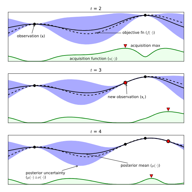
figure example on bayesian optimization$^{[7]}$
suppose
we are trying to optimize a single hyperparameter which we have displayed on the x-axis.
and also we suppose that there is an objective function that we want to minimize and this is displayed on the y-axis
the dots denote what we have observed before
what we do in bayesian optimization is we fit a surrogate model to these observations which is going to predict the objective function value for the hyperparameter value x
the curve here is the mean and the shaded areas display uncertainty about given points
- at point at which we have directly evaluated or observed the real or underlying objective function, the uncertainty is zero
- so we can see in the point, the uncertainty is very low. as we move further and further away from observation, the uncertainty around the predictions actually increase which is logical because we have not explored points in that area.
once we have the model, we can compute acquisition function which tell us how promising different areas of this hyperparameter space are
- once we have computed this we can actually select new points accordingly
- as the uncertainty increases, the acquisition function also tends to increase a bit
pros
- scalability => do not typically scale well to high dimensions and exhibit cubic complexity in the number of data points
- flexibility => do not apply to complex configurations spaces without special kernels
- robustness => require carefully-set hyper-priors
SMAC
as we mentioned before, if we use Gaussian process as the surrogate model, it can only support numerical hyperparameters. as for other SMBO algorithm, they all have 3 key limitations
- only support numerical hyperparameters, which is the same as GP
- only optimizes target algorithm performance for single instances
- lacks a mechanism for terminating poorly performing target algorithm runs early (except successive halving and its extension hyperband)
in order to address first two limitation, SMAC thus make SMBO applicable to general algorithm configuration problems with many categorical parameters and sets of benchmark instances
idea
suppose there are some sampled configurations with their performance under fixed dataset, ${ (x_1, f(x_1)), (x_2, f(x_2)), \dots, (x_n, f(x_n)) }$.
what SMAC do is do fit a model $f$ based on random forest, it’s likened to a multidimensional normal distribution formed by n observations in the Gaussian process.
since random forests can handle discrete variables, this method naturally lends itself to cases where the variables are discrete (categorical). for scenarios involving conditional constraints, it is only necessary to incorporate these constraints into the parameter space to ensure that certain impossible situations are not sampled.
modeling process
in the Gaussian regression process, for a newly added point x forming a new multidimensional normal distribution with previous points, solving the marginal distribution of the newly added point yields its mean and standard deviation.
how is this achieved in the random forest model is that for a new point x, there is a prediction result on each tree in the random forest. averaging the prediction results of all trees yields the mean, and calculating the standard deviation of the prediction results gives the standard deviation.
another advantage of random forests is that for a point x, the prediction complexity on each tree is only $O(logN)$, whereas in the Gaussian regression process, complex matrix multiplication is required to obtain the mean and standard deviation.
next observation
- select the top 10 points in the current data set that maximize the acquisition function as starting points
- find neighboring points using the random neighbors method, and make predictions using the random forest model.
- random neighbors for a specific point =>
- randomly switching the values of all its discrete variables
- sampling the continuous variables with a mean equal to the current value and a standard deviation of 0.2 (continuous variables were normalized to [0,1] beforehand)
- by randomly sampling 10,000 points using this method, predicting their mean and standard deviation with the random forest
- calculating the acquisition function, and selecting the point with the highest value as the next iteration point
TPE
tree parzen estimator
definition
instead of modeling the performance of given hyperparameter value $p(y \vert x)$, what we do in TPE is that we model the opposite
- model the probability of observing a given hyperparameter value x given a certain loss value (or performance)
- $p(x \vert y)$
- x = value of single hyperparameter
- y = loss (performance)
maintain two surrogate models
- a distribution for bad values => $p(x \vert y > y^*) = p(x \vert bad)$
- $p(x \vert y > y^*)$ means the probability distribution over the hyperparameter values given the loss y was worse than the threshold $y^*$ that we have determined
- also can write as the probability of observing hyperparameter value when given that the performance is bad
- a distribution for good values => $p(x \vert y \leq y^*) = p(x \vert good)$
- here the threshold determines good/bad split and it’s determined by hyperparameter $\gamma$
- suppose have 100 different observations and the gamma is set to 0.5, this means that we take the best 50 observations in order to fit the good distribution and we use the 50 worse to fit the bad distribution
get new promising candidates => a promising candidate is likely to
- have low probability under the bad distribution $p(x \vert bad)$
- have high probability under the good distribution $p(x \vert good)$
- promisingness $\varpropto \frac{p(x \vert good)}{p(x \vert bad)}$
- the promising score of a hyperparameter value x can be computed as the ratio between these two probabilities
- according to the equation, promisingness score increases when the probability under the bad distribution is low or the probability under the good distribution is high
- this result is actually proportional to the expected improvement (EI)
- the author use this promisingness to take place of normal EI as a new acquisition function
example
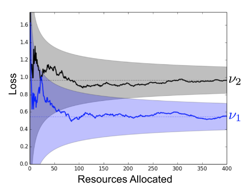
the blue plot denotes the objective function we want to minimize and there are some points we have observed for the good group and bad group accordingly.
what TPE do is to fit a probability distribution for the good observations (green circle) and one for the bad observations (orange cross)
the second image shows these two distribution we fit. here EI denotes no longer normal EI but the promisingness we have defined using two distributions before
we can find that the probability of the bad group is higher at the point where we have actually made observations (approximately x = 0.5 in the second image), so we will not select history observations as the next new observation since in this iterate it’s promisingness is quite low due to the high probability under the bad distribution
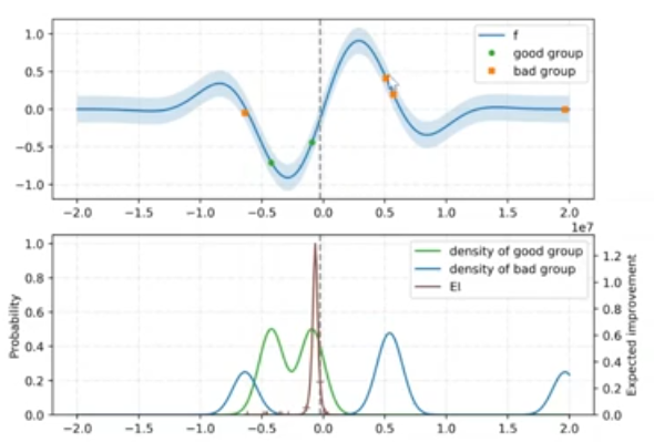
after we have chosen the configuration we want to evaluate next (maximum value of EI, approximately -0.1 in the image), we now again compute our good and bad group based on the value of gamma (re-evaluate which point belong to the good group and which point belongs to the bad one), and again fit the two distributions, then compute the expected improvement again
types of distribution used
depends on the type of the hyperparameter
- categorical => categorical distribution (point mass frequency)
- real-valued/integer
- sample in original space => mixture of truncated Gaussians
- sample in log-space => mixture of truncated Gaussians in log-space
- what is the mixture really is
- why should use truncated distribution => in the previous hyperparameter optimization as well as in random search we actually specify the admissible range of values over which we want to search and we want to be able to do the same for TPE, so we want to be able to say this is the minimum value or this is the maximum value and go find something in between. By truncating these distributions we can enforce this constraint so that the values outside of this range automatically get assigned a probability of zero
about mixture
suppose there are 3 observations
what TPE does is that it’s going to fit a Gaussian to every one of these points.
- so every observation will get a Gaussian fitted to it with the mean equivalent to its hyperparameter value.
- the standard deviations of these Gaussians set are equal to the maximum distance between the right or the left neighbor
after every value have their own different Gaussian distribution, now we can mix these distribution in order to end up with a single distribution
if we want to compute the mixture probability density at a point, we just need to first compute its density under each original Gaussian distribution and then normalize by the number of gaussians so that it stays a valid probability
cons
- easily supports mixed continuous and iscreate spaces due to the nature of kernel density estimators
- model construction scales linearly in the number of data points in contrast to the cubic-time Gaussian processes predominant in the BO literature
BOHB
- vanilla bayesian optimization is typically computationally infeasible
- Bandit-bansed configuration evaluation approach based on random search lack guidance and do not converge to the best configurations as quickly
what bohb to do is to combine the benefits of these two methods (in particular, hyperband)
=> model-based hyperband, strong anytime performance and fast convergence to optimal configurations
idea
BOHB relies on HB to determine how many configurations to evaluate with which budget, but it replaces the random selection of configurations at the beginning of each HB iteration by a model-based search
- once the desired number of configurations for the ieration is reached, the standard successive halving procedure is carried out using these configurations.
- we keep track of the performance of all function evaluations $g(x, b) + \epsilon$
- here $x$ denotes configurations
- $b$ denotes the budget
- and $\epsilon$ denotes the basis of the model
algorithm
closely resembles TPE, with only one major difference.
Image below shows the initial configuration selection procedure of BOHB
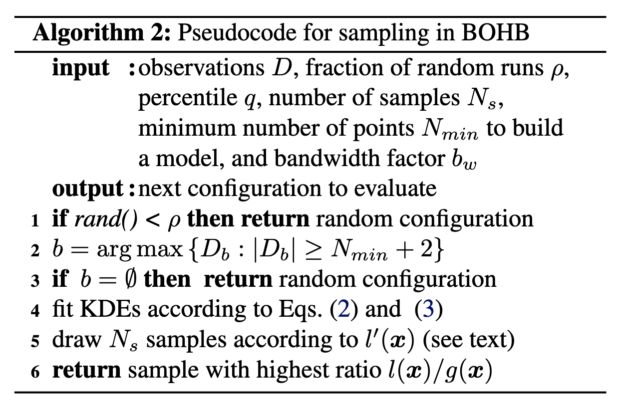
here
$d$ denotes the number of hyperparameter
$N_{min}$ denotes the minimum number of data points to build the selection model, in this paper the author set to $d+1$ for experiments
$\vert D_b \vert$ denotes the number of observations $D$ of the input for budget $b$
$l(x) = KDEs$, $l’(x) = b_w · l(x)$
Promisingness = $\frac{l(x)}{g(x)}$
Then
we opt for a single multidimensional KDE compared to the hierarchy of one-dimensional KDEs used in TPE in order to better handle interaction effects in the input space
- so the keypoint here is to fit a useful KDEs
to build the model as early as possible, we do not wait until $N_b$ equal to the number of observations $\vert D_b \vert$ for budget $b$ which we input.
instead, we initialize with $N_{min} + 2$ random configurations first
we set
- $N_{b, l} = \max (N_{min}, q · N_b)$ where $q$ denotes the percentile which is the input of the algorithm
- $N_{b, g} = \max (N_{min}, N_b - N_{b, l})$
- here the first one denotes number of best configurations and the second denotes the worst one, since we use TPE method as the BO part
- this step is equal to re-evaluating good points and bad points in TPE
then we fit the KDEs ( $l(x)$, $g(x)$ ) according to the TPE method and $N_{b, l}, N_{b, g}$
- this step is equal to model the densities (fit two distribution) in TPE
after we fit the $l(x)$, we need to determine the configurations sampling parameter according to $l(x)$, we do not use $l(x)$ directly, instead
- we multiply it by a factor $b_w$ to encourage more exploration and we call it $l’(x)$
- then we sample $N_s$ points from $l’(x)$ as the sampling result
- keep track of the promisingness and its sampling result of this iteration
return the sampling results with highest ratio (promisingness)
references
- AutoML: A survey of the state-of-the-art
- https://zhuanlan.zhihu.com/p/139605200
- Bergstra, J., Bardenet, R., Bengio, Y., and Kégl, B. Algorithms for hyper-parameter optimization. In Advances in Neural Information Processing Systems, 2011.
- Hutter, F., Hoos, H., and Leyton-Brown, K. Sequential modelbased optimization for general algorithm configuration. In Learning and Intelligent Optimization, volume 6683, 2011.
- D.R. Jones. A taxonomy of global optimization methods based on response surfaces. Journal of Global Optimization, 21:345–383, 2001.
- J. Villemonteix, E. Vazquez, and E. Walter. An informational approach to the global optimization of expensive-to-evaluate functions. Journal of Global Optimization, 2006.
- N. Srinivas, A. Krause, S. Kakade, and M. Seeger. Gaussian process optimization in the bandit setting: No regret and experimental design. In ICML, 2010.
- A Tutorial on Bayesian Optimization of Expensive Cost Functions, with Application to Active User Modeling and Hierarchical Reinforcement Learning
- amieson, K. and Talwalkar, A. Non-stochastic best arm identification and hyperparameter optimization. In Conference on Artificial Intelligence and Statistics, 2016.
- Li, L., Jamieson, K., DeSalvo, G., Rostamizadeh, A., and Talwalkar, A. Hyperband: Bandit-based configuration evaluation for hyperparameter optimization. In International Conference on Learning Representations, 2017.